

How To Use A Pivot Table In Excel -
If you're working with a lot of data in Excel, you know how time-consuming it can be to sort through and analyze all that information. But with a pivot table, you can quickly and easily summarize your data and look at it in different ways. Here are some tips, ideas, and how-tos for using pivot tables in Excel.
What is a Pivot Table?
Definition
A pivot table is a powerful tool in Excel that allows you to summarize, analyze, and present your data in a clear and concise way. It allows you to easily group and filter data, calculate sums and averages, and create charts and graphs based on your data.
How to Create a Pivot Table in Excel
Step 1: Organize your data
The first step to creating a pivot table is to organize your data in a table format. Each column should have a heading, and each row should be a separate record. Make sure that there are no blank rows or columns in your data set.
Step 2: Select your data
Next, select the data range that you want to include in your pivot table. Make sure that all the columns have headings, and that there are no blank rows or columns in your selection.
Step 3: Insert the pivot table
Click on the "Insert" tab, and then click "Pivot Table" in the "Tables" group. Select the range of data that you want to use for your pivot table, and then choose where you want to place the pivot table on your worksheet.
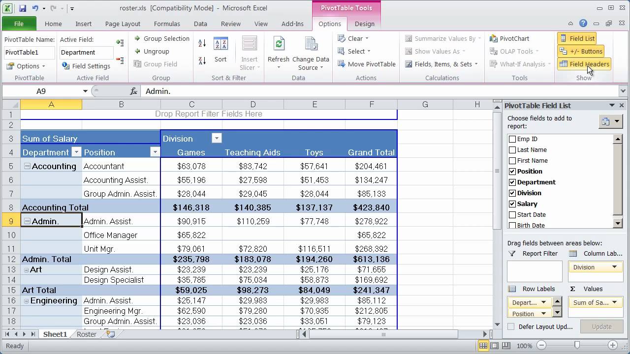
Step 4: Customize your pivot table
Once you've created your pivot table, you can customize it to suit your needs. You can choose which columns to display, apply filters to your data, and create calculated fields and items.

Tips for Using Pivot Tables in Excel
Tip #1: Use Slicers to Filter Your Data
Slicers are a powerful tool in Excel that allow you to visually filter your pivot table data. With a slicer, you can quickly select the data that you want to view, and then see the results in your pivot table.
Tip #2: Use Grouping to Summarize Your Data
You can use the grouping feature in Excel to summarize your data by date, month, quarter, year, or even by hour. This makes it easy to analyze trends and patterns over time.
Tip #3: Use Calculated Fields to Create Custom Formulas
If the built-in Excel functions aren't enough for your needs, you can create your own custom formulas using calculated fields. This allows you to perform complex calculations based on your data.
Ideas for Using Pivot Tables in Excel
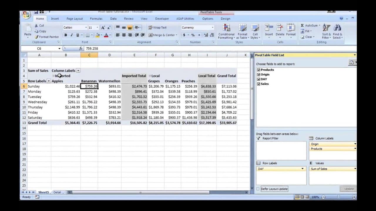
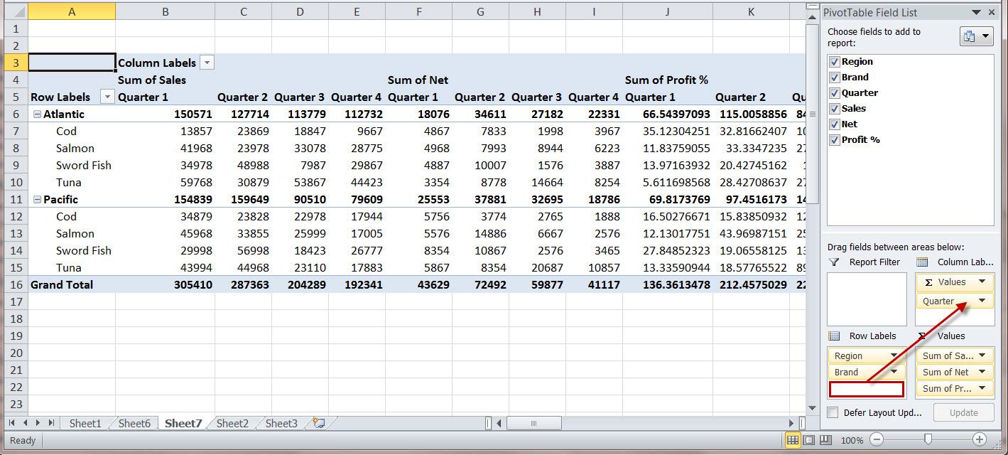
Idea #1: Analyze Sales Data
If you're working in sales, a pivot table can help you analyze your sales data by region, product, or customer. This can help you identify your best-selling products, your most profitable customers, and your top-performing sales reps.
Idea #2: Analyze Survey Data
If you're conducting a survey, a pivot table can help you analyze the data by question, response, or demographic. This can help you identify patterns and trends in the data, and make data-driven decisions based on the results.
Idea #3: Analyze Website Traffic Data
If you're running a website, a pivot table can help you analyze your traffic data by page, source, or user. This can help you identify your most popular pages, your most effective marketing channels, and your highest-converting user segments.
Conclusion
Pivot tables are a powerful tool in Excel that can help you quickly and easily summarize and analyze your data. With a little practice, you can use pivot tables to gain valuable insights into your data and make data-driven decisions based on the results.
So, start organizing your data today and try creating your own pivot table in Excel. You'll be amazed at how easy it is to get started, and how much you can learn about your data with just a few clicks.
Special Mention:
If you want to learn more about pivot tables and how to use them in Excel, check out the Top 3 Tutorials on Creating a Pivot Table in Excel.
Find more articles about How To Use A Pivot Table In Excel